In this ongoing series, the author tries to explain how to use a black box – a neural network configured as a GAN (or generative AI in popular terms) – to program a brown box – The infamous Yamaha DX7 synthesizer.

To the first post of the series: Deep DX – Creating DX7 sounds with AI: Part 1 – Introduction

Factor in some Refactoring

Apologies for the bit of radio silence, but I have been busy rewriting the framework, converting it to use PyTorch instead of Keras/Tensorflow. Why, you might ask? Well, I wanted to give myself the challenge of learning another popular framework, and I also prefer the syntax of PyTorch, which is purely a subjective matter of preference, of course.

As with most renovations, things took longer than expected, and add in a few real-world distractions – and here we are now.

The upside is that the neural net still generates useful sounds – sometimes perhaps a bit too harsh, and sometimes surprisingly beautiful – so nothing has been broken. I did take some time to experiment once again with using different network architectures, but the results were, if anything, still somewhat baffling.

Dancing About Architecture

Whoever uttered the famous quip “writing about music is like dancing about architecture” should try describing the inner workings of a generative network. In fact, even choosing the inner workings can be confounding.

The discriminator consists of a number of layers condensing the 16×16 data representation of a DX7 patch into a resulting vector of 100 values in the range [-1, 1]. As we only want to train the discriminator to sort out “bad” patches from “good” we don’t care about the categorization that is used to label patches when generating.

The generator somewhat mirrors the discriminator, using deconvolution of course to go from a random vector and a wanted category. As this is a CGAN, a category vector was appended to the input noise for the generator, where the eight sound classes I derived from mining the patch data are represented with an integer value in the range [0,7] which is mapped to a feature vector of size 50 before being fed into the generator. Leaky ReLU activation was used in each step, apart from the last, where tanh was used.

Why did I end up with this architecture? Does this represent the optimal topology into which to encode the inner workings of a DX7 patch? I wish I could say “yes”, but I have to disappoint you by admitting to quite a bit of trial and error before finally ending up with this architecture, which seems to work surprisingly good.

As it turns out, finding the proper architecture seems to be a bit of black magic. The consensus of the research papers I read so far seems to indicate that while there are a lot of good ideas on how to structure your network, you still have to test different topologies until you find something that works. When it doesn’t work, which was the majority of early attempts, the network either fails to stabilize entirely, or it falls prey to mode collapse.

Collapsing New People

Mode collapse occurs when the GAN fails to produce a full range of possible outputs, instead stabilizing around only a few plausible variants (or as in the example above, exactly one sound – which quickly becomes boring albeit being quite a good patch…) While not exactly exciting, this was still a much preferable option to the dreadful squeals produced by generators failing to stabilize around reasonable sets of values. (My strictly non-scientific speculation from years of synthesizer programming is that 99.9% of all parameter combinations in FM synthesis invariably leads to more or less unmusical recreations of some of the most dreadful sounds you can imagine, showered in frequencies that will upset cats and dogs alike)

An interesting thing I noted in my experiments was the realization that sometimes less is more. By this I mean that adding layers or dimensions to the network didn’t have the effect of the network being able to learn faster or produce more intricate patches. Indeed, sometimes the opposite seemed to be the case. Also, feature map size and stride were parameters I tinkered quite a bit with during my experiments. For the discriminator I eventually settled on a feature map size of 2 by 2 for all layers expect the first one (4×4), and a stride of 2 for all layers expect the final fully connected one of course. For the generator, three layers of 2×2 seemed to do the trick, in 128 dimensions.

Feature map size corresponds to the size of every feature detection matrix scanning the input, and stride is simply the amount of data points (or pixels in the case of an image) the filter is shifted at each iteration of a pass over the input data. Interestingly, I could never get good results with feature maps of an odd size (such as 3×3), but I will continue the experiments.

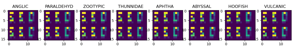
Again, here are examples of visualized patches, real ones to the left (from the training data) and generated ones on the right.

More on Algorithms

In the previous article, we touched upon the strategy devised to deal with the discontinuities in sound introduced if the algorithm is changed. The way I chose to do it, was to train a separate model for each algorithm. This means that the training data is split up according to algorithm, and then categorized individually, according to sound type.

An obvious problem is that splitting the training data reduces the amount of available data to train on, which will have a negative impact on the results. Thus, I opted to group several algorithms together and pool their patch data. The grouping was made according to how similar the algorithms were structurally, so patches from algorithms 1 and 2 are pooled, as they both consist of two columns of operators, one with a carrier and a single modulator, and the other with three modulators, the only difference between the algorithms being where feedback is applied (operator 2 or 6 respectively).

This increases the amount of training data, but also represents a tradeoff in precision as data from two slightly different algorithms is now combined to represent one of them. From the results, I believe the tradeoff is necessary. This means that in the end, six models were trained, each corresponding to a particular group of similar algorithms, and when generating sounds, heuristics based on the data statistics determine which model is used for generating sounds from different categories.

This map shows the number of patches of a particular category vs. algorithms used, and is very useful for understanding the distribution of sounds and algorithms.

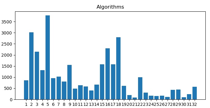
And finally, to answer the question posed in the last part – which is the most commonly used algorithm? The answer can be seen below, and is perhaps not too surprising, at least not to a seasoned DX7 programmer!