The ongoing series where we explore how to create sound patches for the Yamaha DX7 synthesizer using machine learning, or “AI”.

The patch format for the DX7 basically consists of a number of values, all of which are interpreted by the internal circuitry as parameters to generate a sound. As FM synthesis is by definition a mathematical process, many of these act as parameters to the mathematical function(s) for creating the actual sound, while others shape the sound over time through manipulating said parameters through LFO’s and envelopes. (If you really want to dive deep into the somewhat surprising ways in which the DX7 actually does this in hardware, you don’t want to miss Ken Shirriff’s amazing blog where he dissects the DX7 internals)

These are also the values needed to parametrize our neural network in order to (first) train it, and (later) generate new combinations for useful sound patches. As one of my requirements for this experiment was to be able to run training locally on my Mac Studio M1, I started by trying to find the minimal subset of parameters by weeding out data that have less useful or minimal impact on the final sound. (I can always add them later, should I want to)

Obviously, all parameters regarding frequencies and levels for the six operators are to be considered non-expendable, as are the (level) envelopes. For a single operator, the bare minimum would consist of output level, frequency settings (coarse/fine) and velocity sensitivity (although strictly not necessary for the actual resulting sound, I find this a vital part of the expressiveness of FM sounds)

class DXOperator:
    def __init__(self):
        self.out = 0
        self.fc = 0
        self.ff = 0
        self.vs = 0

Six operators would yield 24 parameters so far. After pondering the other parameters, I opted to add detune which brought the total up to 30. (Why detune? Because it’s also one of those small but important parameters that can breathe life into an otherwise static sound, and I was curious to see how many of the existing patches used detuned operators to any extent)

Next up are the envelopes. Each of the six operators has a volume envelope, and every envelope consists of eight parameters: Four levels and four rates.

class DXOperator:
    def __init__(self):
        self.r1 = 0
        self.r2 = 0
        self.r3 = 0
        self.r4 = 0
        self.l1 = 0
        self.l2 = 0
        self.l3 = 0
        self.l4 = 0
        self.dt = 0
        self.out = 0
        self.fc = 0
        self.ff = 0
        self.vs = 0

This now brought the total up to 13*6 = 78 parameters. In the first versions of the software, I chose to omit the following parameters:

• Keyboard level breakpoint, left and right keyboard level scaling and curve
• Keyboard rate scaling
• Oscillator mode (I simply set it default to “ratio”)
• Transpose

I also decided to omit the Pitch Envelope parameters, as they are global for the patch rather than per operator. The way Yamaha designed Pitch Envelope and Pitch LFO seriously hampers the potential for sound design, and in my eyes reduces pitch modulation to special effects, but I assume it was one of several cost-cutting compromises made during the design of the instrument. Indeed, already in the SY77, you have the opportunity to add pitch modulation to individual operators. Thus, I did not include it in my software.

class DX7Patch:

    def __init__(self):
        self.name = ""

        self.op = [0, DXOperator(), DXOperator(), DXOperator(), 
                      DXOperator(), DXOperator(), DXOperator()]

        self.algo = 0
        self.fb = 0
        self.transpose = 24

Adding the global parameters of a patch, name, algorithm number, transpose and feedback (which is always just one value no matter the algorithm in the DX7), we end up with a grand total of 78 + 2 = 80 parameters to train and test! (I opted not to include name or transpose data as they can be heuristically generated). This makes for a reasonably sized dataset, and indeed it turned out that I could train 400 epochs in a matter of minutes each time.

Now that the relevant parameters were selected, how would they best be represented? From my early experiments with Deep Learning and image generation back in 2015 I am quite familiar with scanning images through convolution kernels, and I wondered if this would be a feasible technique for DX patch data as well? I found a few recently published papers that seemed to show promise for using convolution kernels onto a 2d mapping of non-image training data, so I decided to give it a shot, meaning that I could apply all my previous knowledge of convolutional neural networks, or CNN’s for short to this problem. A consequence of this was that I now had to find a way to map the patch data into a 2d space that would enable a CNN to learn how to recognize important features from patches.

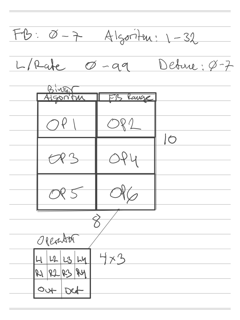
This turned out to be an interesting exercise. My first attempt can be seen as sketched in my digital notebook in the picture. The “image” can be visualized as six blocks of 4 by 3 pixels where each value is encoded to a normalized [0,1] float representing its full range. (This is later expanded to the range [-1, 1] for training reasons)

By zooming in on an individual operator, output and detune values are repeated across two pixels, to create a rectangular shape (wholly unnecessary, as I found out later) and Feedback is represented in a similar way, “tacked” on to the rightmost stack of operators, whereas the Algorithm parameter was encoded as a binary representation (four bits) across the left hand stack.

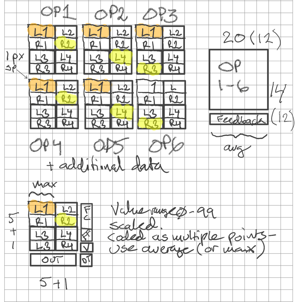
This was fairly quickly updated to a modified representation, where frequencies and velocity mod level was added (right). This became the first representation of patch data that I performed actual training on. Results were inconclusive.

As anyone who has experimented with Generative Adversarial Networks can attest, they are temperamental, and getting them to a point where the training stabilizes sufficiently without suffering from mode collapse or other problems is often a game of trial and error.

One of the things to note about the implementation above, is that I had the idea that it would prove beneficial to keep things symmetrical. For this reason, some parameters (for instance Feedback and Frequency Coarse above) were distributed over multiple pixels, with the average value taken as the actual result. (And if you are wondering, no, it didn’t provide any benefits whatsoever, and was removed for the final version)

We will look at the different network architectures later, but suffice to say, I tried quite a few different setups, with poor results. Patch generation was a mixed bag, with a few playable gems awash in a sea of FM nastiness. My cat, who in general prefers to be within arms length of me when I work from home, took offense in the obnoxious overtones and retreated to another floor.

So, I tried another setup, where I had the idea of separating the envelope data from frequency and other parameters. Thus, the six operators’ envelopes were followed by their respective frequency data (coarse followed by fine), output levels, etc.

The idea behind this was to group frequency relationships apart from timing (envelope) relationships to see if the GAN could find features easier from this representation.

As it turned out, it actually performed worse than the previous format. (I am sure there’s a mathematical reason for it, and someone can probably explain it better – I can only guess at the reasons)

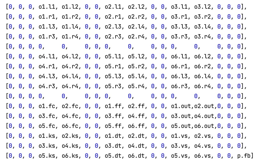
The third version, depicted to the right in its final form, where key level scaling and other data had been added, clustering all relevant data per operator together, gave promising results almost immediately, and I could now focus on finding the right architecture and fine tune the training parameters.

Apparently, it was easier for the GAN variants to find relevant features when comparing operators, than when grouping data according to the different parameter types.

One final item to note is the absence of the Algorithm parameter. Why wasn’t it also included in the training set?

That will be explained in the next installment!